Second, generate world or random cities, and then adjust the names and locations of the cities, by clicking on a city and adjusting its time zones and latitudes. Time zones are represented relative to Greenwich Mean Time, so London is "0" and U.S. Eastern Time is "-5". They are used to estimate longitude. Latitude may be set as well, but is merely used for realism and to prevent overlap, and has no impact on model results. Time zone selections may impact model results, due to "follow the sun" efficiencies.
Third, select a distribution for each city, and the maximum and minimum server count for each city and distribution. The default distribution is "uniform," but other distributions, such as those modeling "workers" or "daily" cycles may be more appropriate. A city may be turned "off" by selecting "none."
Fourth, compare the difference between non-pooled and pooled resource capacity requirements. Pooling will never result in a greater capacity requirement, and may result in dramatically lower requirements globally.
Lastly, click on "Data" to review the raw data, and then possibly import it into a spreadsheet for further analysis. The same data may be viewed graphically by clicking on "Graph," illustrating the individual max capacities, or by clicking on "Stack," showing the compression that results from pooling.
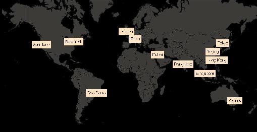
Based on the number of cities selected, either "World Cities" may be clicked to show several major cities (New York, London, Paris, Hong Kong, etc.) or "Random Cities" may be clicked to generate cities uniformly distributed across time zones and latitudes. (Note that some cities may be floating!) Clicking "Random Cities" repeatedly will regenerate cities, and automatically recalculate results so that a range of results may be assessed. San Jose, London, and Hong Kong are spaced 8 hour time zones apart, and consequently have non-overlapping workdays.
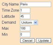
Once the cities have been determined, their attributes may be edited. For example, "New York" or "City3" may be changed to, say, "Oslo," its time zone and latitude changed accordingly, and its local demand distribution and range be changed. Available distributions include:
Uniform Demand -- Uniformly distributed between min servers and max servers.
Normal Demand -- Normally (i.e., Gaussian) distributed, with a mean halfway between min servers and max servers, six standard deviations between min and max, and clipping to ensure that results are no smaller than min and no larger than max. (Note: The Box-Muller Transform is used to generate normally distributed values)
Worker Demand -- 0 after hours, but uniformly distributed weekdays from 9 to 5, in the local time zone.
Gamer Demand -- Gamers are assumed to have day jobs (and therefore have a demand of "0" during the workday), but are active nights and weekends, again, in the local time zone.
Daily Demand -- A cycle which peaks at max servers and diminishes down to min servers, repeating on a daily basis, timed to the local time zone.

The results of an unpooled resource model may be contrasted with a pooled resource model. Changing the distributions, the number of cities, the inter-time-zone spacing, or all of these parameters may demonstrate lesser or greater benefit.
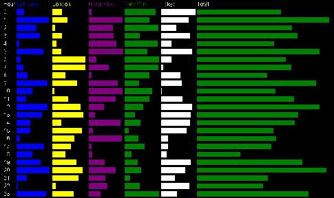
Clicking on "Data" or "View Data" brings up the results in tabular form. The data may be the copied into a spreadsheet for further analysis (Note: copying the data first into a word processor and from there into a spreadsheet may help preserve table formatting). Clicking on "Graph" or "View Bar Graph" brings up a bar graph view of the data. The demand, each hour, in each city, is shown as a bar proportional to the number of equivalent servers worth of demand. The total demand for each hour is also shown, and, at the bottom, the maximum demand required per city.
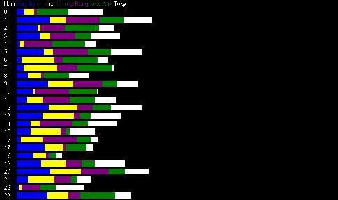
Clicking on "Stack" or "View Stacked Bar Graph" brings up a "stacked" bar chart, that is, the demand each hour is shown as a series of bars that are contiguous, thus illustrating the total demand for that hour as well as the proportion from each city. Contrasting the stacked bar graph with the (non-stacked) bar graph clearly illustrates the ability of resource sharing across the grid to reduce overall capacity requirements, by "collapsing" the demand each hour as tightly as possible