Close Help Window

Overview	This model illustrates the benefits of dispersion for latency reduction, as well as the diminishing returns of additional node builds, leading to a "sweet spot" number of nodes. By "latency," we focus the delay due to travel time, or physical propagation, which we (simplistically for this model), assume to be proportional to "as the crow flies" distance. This model is relevant in scenarios as diverse as locating coffee shops, fast food restaurants, distributed interactive computing environments, and content delivery architectures. In the real world, additional "service time" delays would need to be modeled, such as queueing in routers, or servicing at the node based on load.
Basic Flow	First, select the distribution and quantity of nodes. Nodes may be distributed uniformly or normally across the grid, or arrayed in a lattice. Second, view the distribution graphically of nodes on the map. Third, run any number of random trials, or run a total scan covering the entire grid. Caution: scanning in 1 unit increments on the 100 by 100 grid will chew up your CPU for a minute or so. Lastly, view the results. Latency in many random scenarios should be worse than in a structured lattice, because some nodes are "wasted" being close to other nodes. More nodes should reduce average latency (proxied as distance), but the marginal benefit of each additional node drops off quadratically.
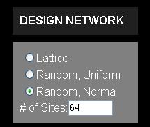
Design the Network	A node distribution may be selected using the radio button, and a total number of nodes from 1 to 256. Structured layouts are available in a variety of regular point lattices: square, equilateral, hexagonal, and isosceles. Square point lattices are indicated by "[]", equilateral by "<|", hexagonal by "<=>", and isosceles by "/".
View the Network	The network may be viewed on the grid, which is 100 units square. Each node is shown as a yellow square.
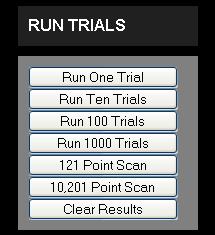
Run Monte Carlo Trials or a Structured Scan	Monte Carlo (i.e., random) trials may be run, or a coarse grained or fine grained scan may be run. Selecting the 121 point scan checks the latency from many points on the grid, in 10-unit intervals, i.e., grid points (0,0), (0, 10), (0, 20), and so forth. Selecting the 10,201 point scan checks the latency from each point on the grid, in 1-unit intervals, i.e., grid points (0,0), (0,1), (0,2), (0,3), and so forth, and may take a minute or so to run, depending on your CPU speed.
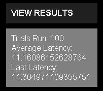
View Results	The number of trials run, the lowest latency (shortest distance to the nearest node) for the most recent trial, and the average lowest latency are shown (i.e., the mean, across all trials, of the distance to the nearest node). The more trials that are run, the more the results will converge to several decimal places. Changing the distribution or number of nodes can help demonstrate the tradeoffs between cost and different layouts. Note: demand in this model is always uniformly distributed in two dimensions across the grid, so normally distributed nodes, typical of say, an urban buildout, will show increased latency rather than accurately reflecting a similarly distributed population of users.
About	This model was written by Joe Weinman in about 500 lines of code, which are a mixture of HTML, DHTML, ASP.NET 2.0 / Visual Basic, stylesheets, and JavaScript, using Microsoft Visual Web Developer 2008. It has been tested in Firefox 2.0 (Mozilla 5), Safari 3.1, and Internet Explorer 7.0. It even runs on an iPhone 3G, at about the same speed as on a laptop, even though most computation is performed on the client.

© 2005-2008 Joe Weinman